What is a Spectrum?

Before we can answer that question we should first discuss a time series briefly. A time series is a sequence of random variables, \(X_{0}, ... , X_{n-1}\), indexed by time with a correlation structure that exists between the different times, \(R(t_{0}, t_{1})\). Order is important, however the indexing variable need not be time, but could be depth (or distance) or any other variable you might want; pressure, brightness, voltage, etc…

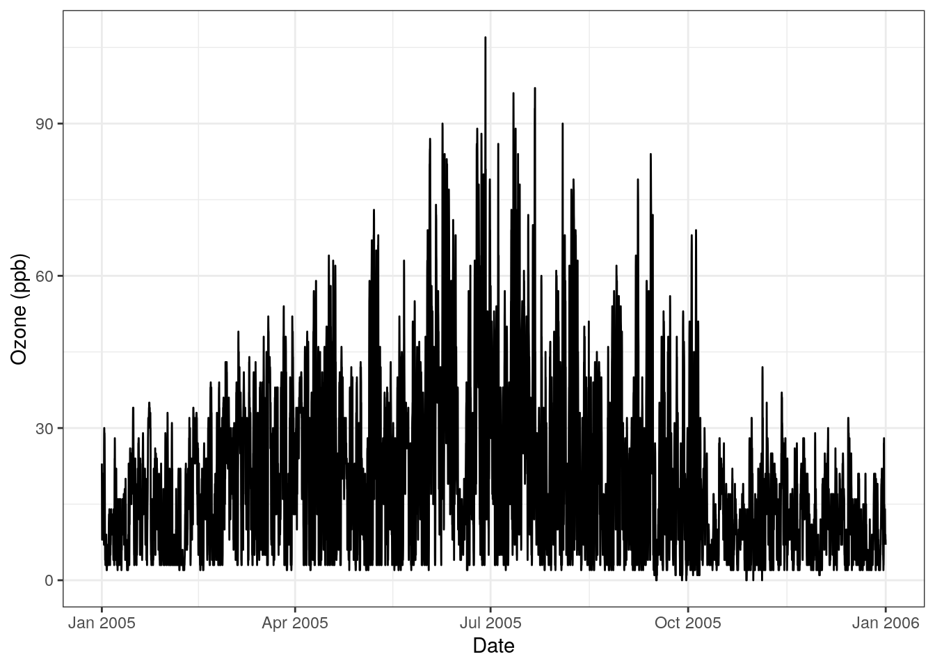
An example of a time series is air pollutation data collected by Environment and Climate Change Canada (ECCC) from their National Air Pollutation Surveillance (NAPS) program. A year of this data is plotted in Figure 1

Figure 1: Ozone time series for NAPS station 60430 located in Toronto, ON.

We will make a few assumptions about our ozone data:

• it is at least weakly stationary
• the distribution of the data does not deviate too far from Gaussian

When a time series is stationary, its distributional properties do not change with time, e.g., the mean and variance are not functions of time.

Neither of these is likely true, however for now we will go with it.

Based on these assumptions we can calculate the autocovariance function (ACVF) of the series:

\[\hat{R}(\tau) = \frac{1}{n-1}\sum_{t=0}^{n-\tau}X_{t}X_{t-\tau}\]

where \(\tau\) is the lag. Because we’ve made the stationary assumption, the ACVF is a function of lag only (remember, the variance (or covariance in this case) is time independent).

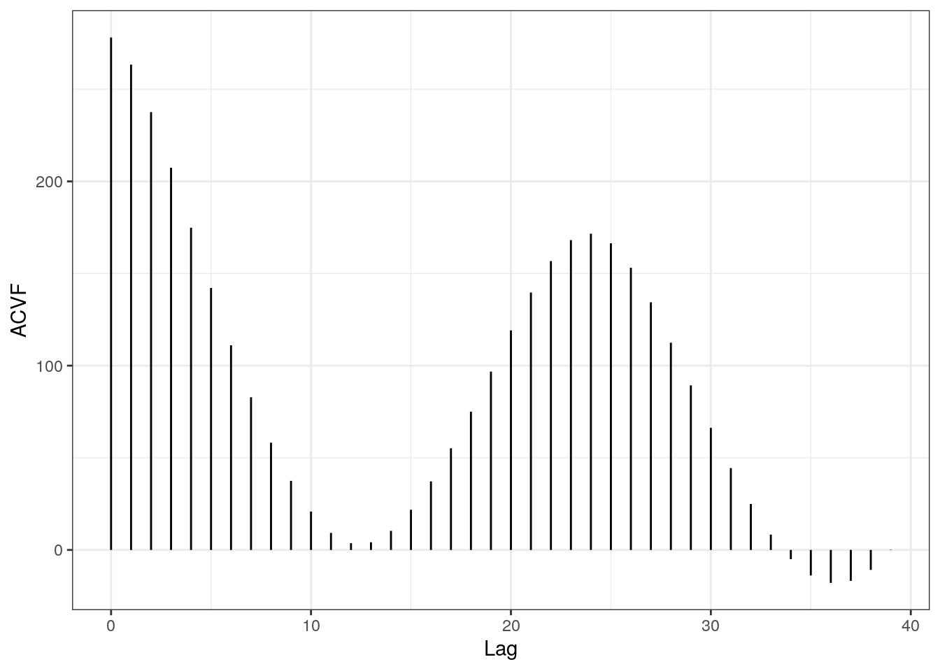
Figure 2: The estimated autocovariance function.

This ACVF in Figure @ref(fig:o3.acvf) is pretty interesting as there appears to be some kind of sinusoidal shape present. We will talk about this in a future post.

It turns out that the spectrum is the Fourier transform of the ACVF, i.e., the spectrum, a function of frequency and denoted \(S(f)\), and the ACVF, \(R(\tau)\), are Fourier transform pairs.

\[S(f) \overset{\mathcal{F}}{\longleftrightarrow} R(\tau)\] We’re getting close - so we know one way to estimate the spectrum, we calculate the sample autocovariance and then Fourier transform it, but what is the spectrum?

The spectrum decomposes the variance of a process by frequency. In other words, we assume that our time series can be represented by a bunch of sinusoids at different frequencies and the spectrum tells us how much variance is contributed by each of these sinusoids. Another way to think about it is which sinusoids are “most important” in the time series.

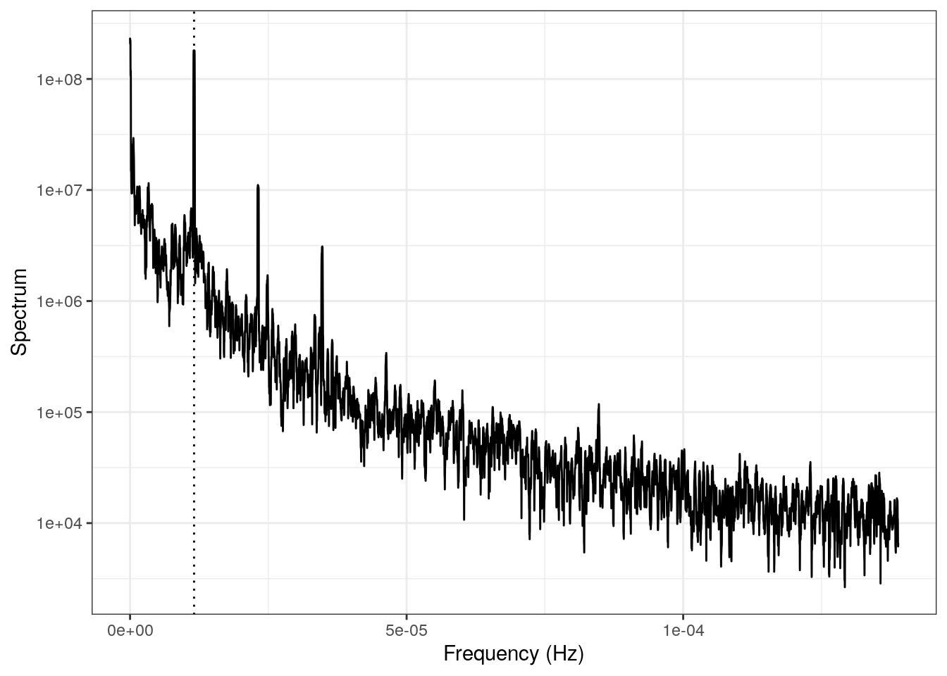
We end this discussion with a quick look at a spectrum (Figure 3) calculated using the Multitaper method (definitely to be discussed in a future post).

Figure 3: The spectrum of the ozone data shown in Figure 1.

This spectrum is pretty interesting in and of itself. From even a quick look it seems that most of the variance in the process is contained in the low frequencies (notice the negative trend). In particular, the frequency corresponding to a period of 1 day (the dotted vertical line) and its harmonics are very prominent, which tells us that there is a strong daily signal contained in this time series. The daily nature of ozone data is unsurprising given the physics / chemistry involved (another post).